Here, we’ll discuss the algorithm for binning data.
By passing the preprocessed 2-D embedding data and hexagonal grid configurations, you can obtain the hexagonal binning information like centroid coordinates, hexagonal polygon coordinates, the standardise counts within each hexagon etc.
hb_obj <- hex_binning(nldr_obj = scurve_model_obj$nldr_obj, b1 = 4, q = 0.1)
## Data set with all possible centroids in the hexagonal grid
all_centroids_df <- hb_obj$centroids
glimpse(all_centroids_df)
#> Rows: 20
#> Columns: 3
#> $ h <int> 1, 2, 3, 4, 5, 6, 7, 8, 9, 10, 11, 12, 13, 14, 15, 16, 17, 18, 19,…
#> $ c_x <dbl> -0.10000000, 0.21223009, 0.52446018, 0.83669027, 0.05611504, 0.368…
#> $ c_y <dbl> -0.08923607, -0.08923607, -0.08923607, -0.08923607, 0.18116312, 0.…
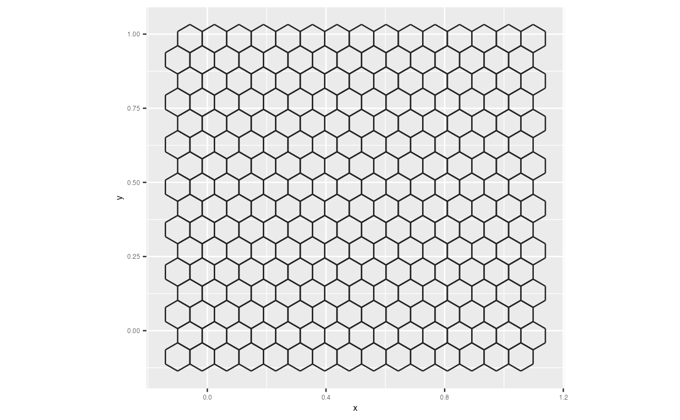
## Generate all coordinates of hexagons
hex_grid <- hb_obj$hex_poly
glimpse(hex_grid)
#> Rows: 120
#> Columns: 3
#> $ h <int> 1, 1, 1, 1, 1, 1, 2, 2, 2, 2, 2, 2, 3, 3, 3, 3, 3, 3, 4, 4, 4, 4, 4,…
#> $ x <dbl> -0.10000000, -0.25611504, -0.25611504, -0.10000000, 0.05611504, 0.05…
#> $ y <dbl> 0.0910300574, 0.0008969943, -0.1793691320, -0.2695021951, -0.1793691…
## To obtain the standardise counts within hexbins
counts_df <- hb_obj$std_cts
df_bin_centroids <- extract_hexbin_centroids(centroids_data = all_centroids_df,
counts_data = counts_df)
ggplot(data = hex_grid, aes(x = x, y = y)) +
  geom_polygon(fill = "white", color = "black", aes(group = h)) +
  geom_point(data = all_centroids_df, aes(x = c_x, y = c_y), color = "red") +
  coord_fixed()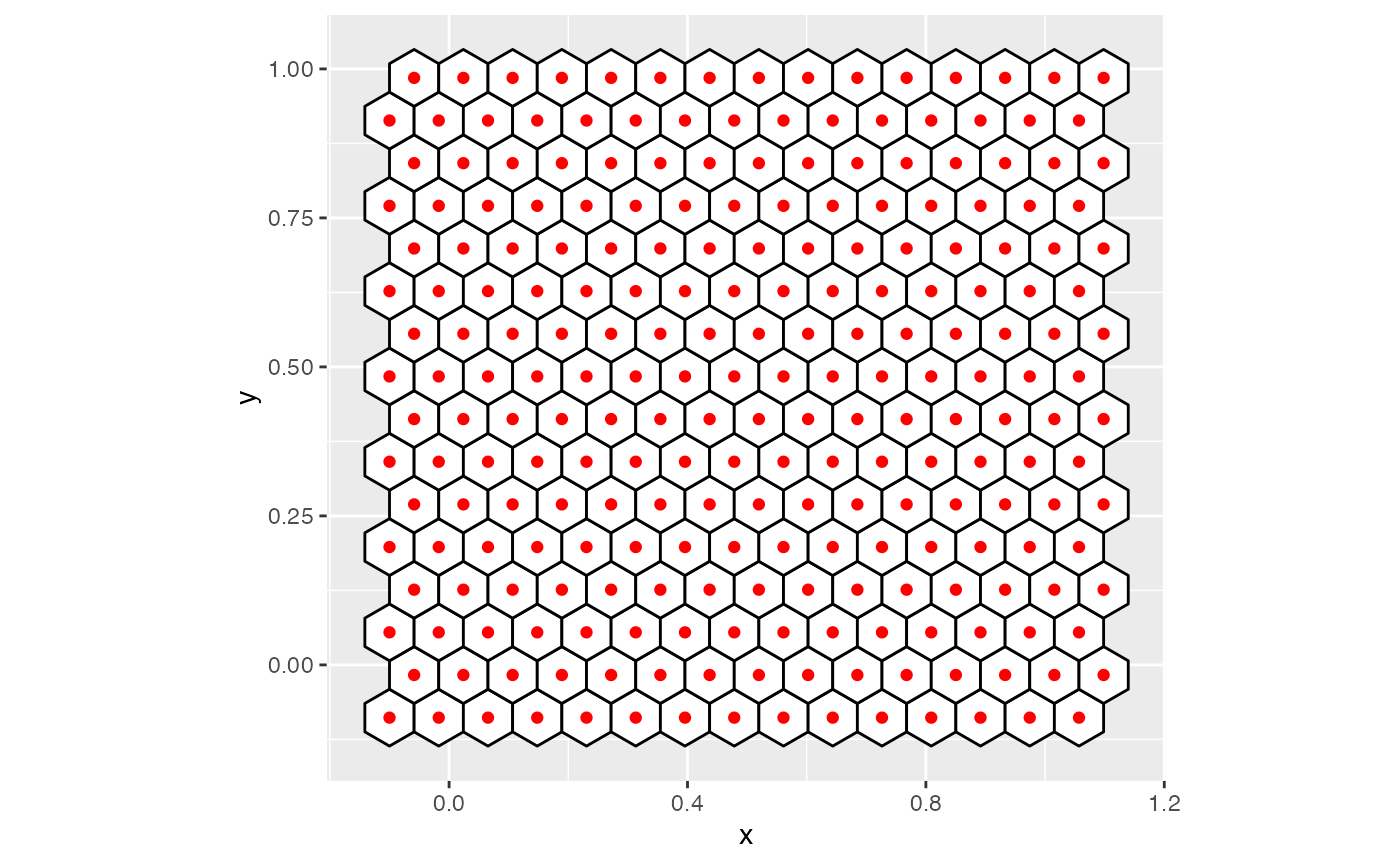
ggplot(data = hex_grid, aes(x = x, y = y)) +
  geom_polygon(fill = "white", color = "black", aes(group = h)) +
  geom_point(data = all_centroids_df, aes(x = c_x, y = c_y), color = "red") +
  geom_point(data = df_bin_centroids, aes(x = c_x, y = c_y), color = "purple") +
  coord_fixed()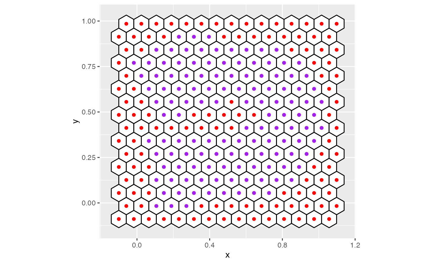
umap_scaled <- scurve_model_obj$nldr_obj$scaled_nldr

ggplot(data = hex_grid, aes(x = x, y = y)) +
  geom_polygon(fill = "white", color = "black", aes(group = h)) +
  geom_point(data = umap_scaled, aes(x = emb1, y = emb2), color = "blue", alpha = 0.3) +
  coord_fixed()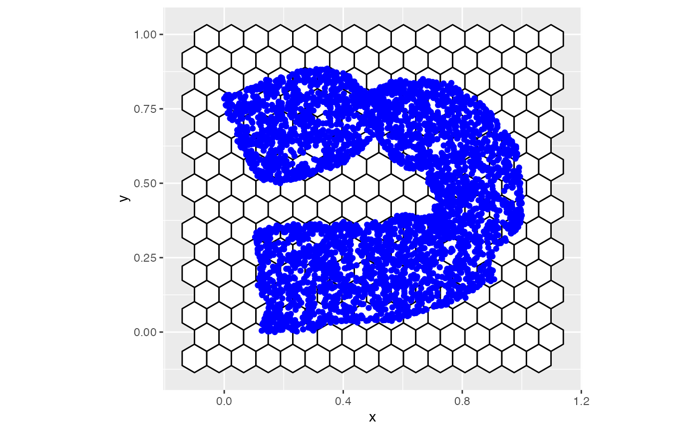
hex_grid_with_counts <- left_join(hex_grid, counts_df, by = "h")

ggplot(data = hex_grid_with_counts, aes(x = x, y = y)) +
  geom_polygon(color = "black", aes(group = h, fill = w_h)) +
  geom_text(data = all_centroids_df, aes(x = c_x, y = c_y, label = h)) +
  scale_fill_viridis_c(direction = -1, na.value = "#ffffff") +
  coord_fixed()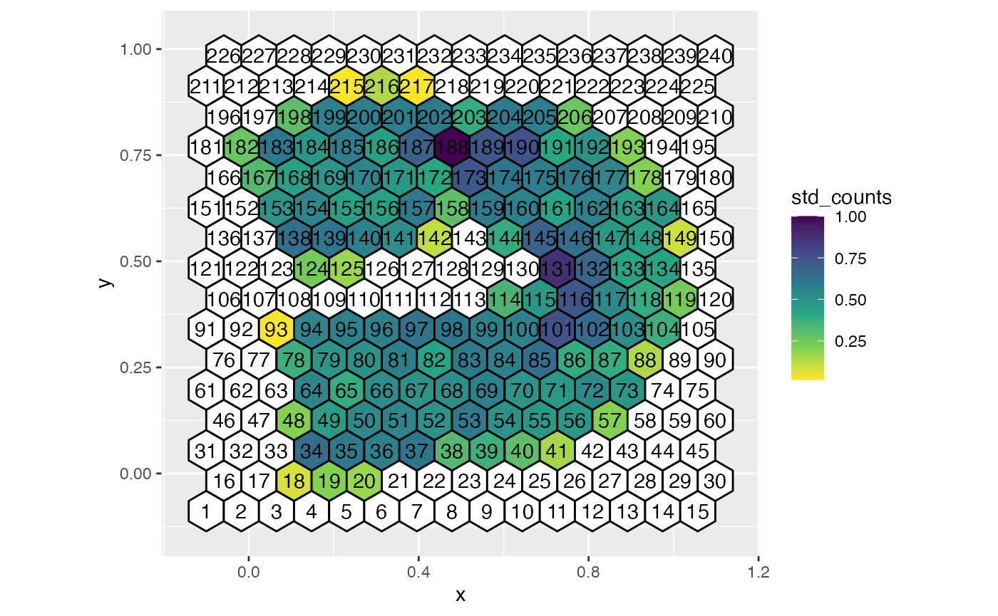
You can also use geom_hexgrid to visualise the hexagonal
grid rather than geom_polygon.
ggplot(data = all_centroids_df, aes(x = c_x, y = c_y)) +
  geom_hexgrid() +
  coord_equal() +
  xlab("x") + ylab("y") +
  theme(axis.text = element_text(size = 5),
        axis.title = element_text(size = 7))