4. Algorithm for visualising the model overlaid on high-dimensional data • quollr

This walks through the algorithm for constructing a model from 2-D embedding data and visualising it alongside high-dimensional data. The process involves two major steps:

Constructing the model in the 2-D embedding space using hexagonal binning and triangulation.
Lifting the model into high dimensions to link it back to the original data space.

library(quollr)
library(ggplot2)
library(tibble)
library(dplyr)
library(stats)

Step 1: Construct the 2-D model

Hexagonal Binning

To begin, we preprocess the 2-D embedding and create hexagonal bins over the layout.

## To pre-process the data
nldr_obj <- gen_scaled_data(nldr_data = scurve_umap)

## Obtain the hexbin object
hb_obj <- hex_binning(nldr_obj = nldr_obj, b1 = 15, q = 0.1)

all_centroids_df <- hb_obj$centroids
counts_df <- hb_obj$std_cts

Extract bin centroids

Next, we extract the centroid coordinates and standardised bin counts. These will be used to identify densely populated regions in the 2-D space.

## To extract all bin centroids with bin counts
df_bin_centroids <- extract_hexbin_centroids(centroids_data = all_centroids_df,
                                             counts_data = counts_df)

benchmark_highdens <- 0

## To extract high-densed bins
model_2d <- df_bin_centroids |>
  dplyr::filter(n_h > benchmark_highdens)

glimpse(model_2d) 
#> Rows: 137
#> Columns: 5
#> $ h   <int> 34, 35, 36, 37, 38, 41, 42, 49, 50, 51, 52, 53, 54, 55, 56, 57, 64…
#> $ c_x <dbl> 0.1502324, 0.2336432, 0.3170540, 0.4004648, 0.4838756, 0.7341080, …
#> $ c_y <dbl> 0.0287916, 0.0287916, 0.0287916, 0.0287916, 0.0287916, 0.0287916, …
#> $ n_h <dbl> 1, 10, 8, 8, 2, 2, 12, 11, 9, 4, 11, 12, 1, 6, 12, 12, 5, 10, 10, …
#> $ w_h <dbl> 0.001, 0.010, 0.008, 0.008, 0.002, 0.002, 0.012, 0.011, 0.009, 0.0…

Triangulate the bin centroids

We then triangulate the hexagon centroids to build a wireframe of neighborhood relationships.

## Wireframe
tr_object <- tri_bin_centroids(centroids_data = df_bin_centroids)
str(tr_object)
#> List of 2
#>  $ trimesh_object:List of 11
#>   ..$ n     : int 300
#>   ..$ x     : num [1:300] -0.1 -0.0166 0.0668 0.1502 0.2336 ...
#>   ..$ y     : num [1:300] -0.116 -0.116 -0.116 -0.116 -0.116 ...
#>   ..$ nt    : int 548
#>   ..$ trlist: int [1:548, 1:9] 1 17 31 16 16 3 33 17 17 46 ...
#>   .. ..- attr(*, "dimnames")=List of 2
#>   .. .. ..$ : NULL
#>   .. .. ..$ : chr [1:9] "i1" "i2" "i3" "j1" ...
#>   ..$ cclist: num [1:548, 1:5] -0.0583 -0.0166 -0.1417 -0.0583 -0.0166 ...
#>   .. ..- attr(*, "dimnames")=List of 2
#>   .. .. ..$ : NULL
#>   .. .. ..$ : chr [1:5] "x" "y" "r" "area" ...
#>   ..$ nchull: int 50
#>   ..$ chull : int [1:50] 1 2 3 4 5 20 35 6 7 8 ...
#>   ..$ narcs : int 847
#>   ..$ arcs  : int [1:847, 1:2] 2 16 1 2 17 16 31 32 16 17 ...
#>   .. ..- attr(*, "dimnames")=List of 2
#>   .. .. ..$ : NULL
#>   .. .. ..$ : chr [1:2] "from" "to"
#>   ..$ call  : language tri.mesh(x = centroids_data[["c_x"]], y = centroids_data[["c_y"]])
#>   ..- attr(*, "class")= chr "triSht"
#>  $ n_h           : num [1:300] 0 0 0 0 0 0 0 0 0 0 ...

Generate edges from triangulation

Using the triangulation object, we generate edges between centroids. We retain only edges connecting densely populated bins.

trimesh_data <- gen_edges(tri_object = tr_object, a1 = hb_obj$a1) |>
  dplyr::filter(from_count > benchmark_highdens,
                to_count > benchmark_highdens)

## Update the edge indexes to start from 1
trimesh_data <- update_trimesh_index(trimesh_data)
glimpse(trimesh_data)
#> Rows: 346
#> Columns: 8
#> $ from       <int> 2, 1, 8, 2, 17, 2, 17, 3, 27, 27, 18, 18, 9, 9, 10, 3, 28, …
#> $ to         <int> 8, 2, 18, 3, 18, 9, 28, 9, 38, 28, 29, 19, 18, 10, 19, 4, 3…
#> $ x_from     <dbl> 0.2336432, 0.1502324, 0.1919378, 0.2336432, 0.1502324, 0.23…
#> $ y_from     <dbl> 0.0287916, 0.0287916, 0.1010275, 0.0287916, 0.1732633, 0.02…
#> $ x_to       <dbl> 0.1919378, 0.2336432, 0.2336432, 0.3170540, 0.2336432, 0.27…
#> $ y_to       <dbl> 0.1010275, 0.0287916, 0.1732633, 0.0287916, 0.1732633, 0.10…
#> $ from_count <dbl> 10, 1, 11, 10, 5, 10, 5, 8, 1, 1, 10, 10, 9, 9, 4, 8, 10, 1…
#> $ to_count   <dbl> 11, 10, 10, 8, 10, 9, 10, 9, 11, 10, 5, 10, 10, 4, 10, 8, 5…

Visualise the triangular mesh

trimesh <- ggplot(model_2d, aes(x = c_x, y = c_y)) +
  geom_trimesh() +
  coord_equal() +
  xlab(expression(C[x]^{(2)})) + ylab(expression(C[y]^{(2)})) +
  theme(axis.text = element_text(size = 5),
        axis.title = element_text(size = 7))

trimesh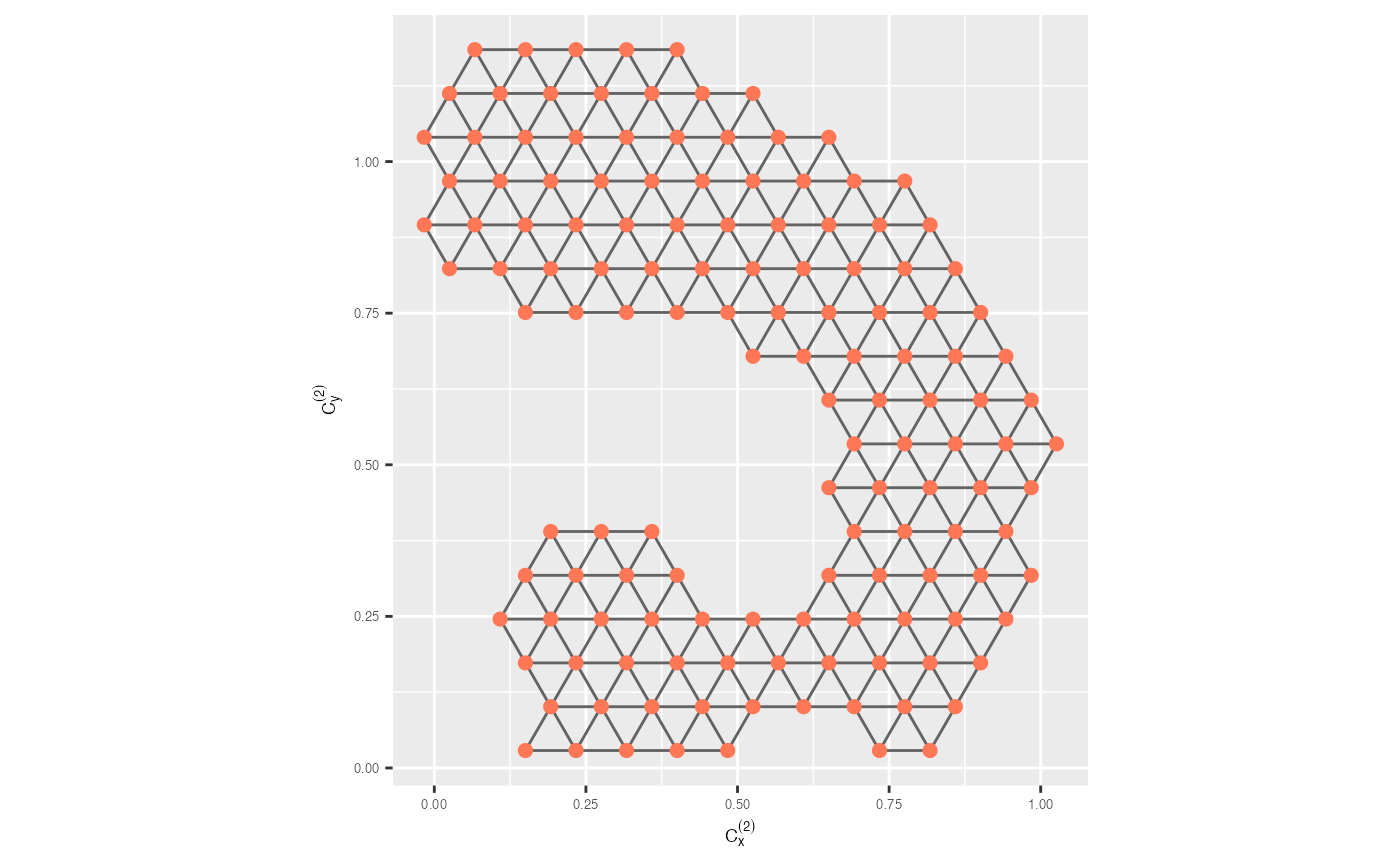

Triangular mesh.

Step 2: Lift the model into high dimensions

Map bins to high-dimensional observations

We begin by extracting the original data with their assigned hexagonal bin IDs.

nldr_df_with_hex_id <- hb_obj$data_hb_id
glimpse(nldr_df_with_hex_id)
#> Rows: 1,000
#> Columns: 4
#> $ emb1 <dbl> 0.27708147, 0.69717161, 0.77934921, 0.17323121, 0.21793445, 0.593…
#> $ emb2 <dbl> 0.91343544, 0.53767948, 0.39861033, 0.95285002, 0.98320848, 1.048…
#> $ ID   <int> 1, 2, 3, 4, 5, 6, 7, 8, 9, 10, 11, 12, 13, 14, 15, 16, 17, 18, 19…
#> $ h    <int> 216, 145, 116, 229, 229, 249, 79, 164, 206, 118, 147, 50, 80, 222…

Compute high-dimensional coordinates for bins

We calculate the average high-dimensional coordinates for each bin and retain only the ones matching the 2-D model bins.

model_highd <- avg_highd_data(highd_data = scurve, scaled_nldr_hexid = nldr_df_with_hex_id)

model_highd <- model_highd |>
  dplyr::filter(h %in% model_2d$h)

glimpse(model_highd)
#> Rows: 137
#> Columns: 8
#> $ h  <int> 34, 35, 36, 37, 38, 41, 42, 49, 50, 51, 52, 53, 54, 55, 56, 57, 64,…
#> $ x1 <dbl> 0.95812568, 0.81844628, 0.54418139, 0.27895124, 0.05667053, -0.3754…
#> $ x2 <dbl> 0.0853925, 0.1158483, 0.1113382, 0.1282115, 0.1193769, 1.5840595, 1…
#> $ x3 <dbl> 1.286348, 1.563969, 1.833843, 1.954630, 1.997485, 1.914399, 1.82979…
#> $ x4 <dbl> 2.650223e-03, 1.842360e-03, -3.414032e-03, 8.798724e-05, 7.325453e-…
#> $ x5 <dbl> 0.0170739819, 0.0036132499, -0.0003026848, 0.0010398644, 0.00238201…
#> $ x6 <dbl> 0.087550004, -0.031822955, 0.019604954, -0.027633204, 0.083256963, …
#> $ x7 <dbl> -0.0024864689, -0.0037675385, 0.0000704427, -0.0002274276, -0.00165…

Step 3: Visualise the high-dimensional model

We now combine all components—high-dimensional data, the 2-D model, lifted high-dimensional centroids, and the triangulation—and render the model using an interactive tour.

Prepare data for visualisation

df_exe <- comb_data_model(highd_data = scurve, 
                          model_highd = model_highd, 
                          model_2d = model_2d)

Interactive tour of model overlay

tour1 <- show_langevitour(point_data = df_exe, edge_data = trimesh_data)

tour1