5. Generating model summaries

This demonstrates how to generate and inspect model summaries. Summarising models fitted to both the high-dimensional space and its corresponding 2-D embedding is an essential step in evaluating how well a low-dimensional representation captures the structure of the original data.

library(quollr)
library(dplyr)
library(ggplot2)

Step 1: Fitting the model

Begin by fitting a high-dimensional model and its corresponding 2-D model using the fit_highd_model() function. This generates the 2-D bin centroids (the 2-D model) and their corresponding coordinates in the high-dimensional space (the lifted model).

model <- fit_highd_model(
  highd_data = scurve, 
  nldr_data = scurve_umap, 
  b1 = 4, 
  q = 0.1, 
  benchmark_highdens = 5
)

df_bin_centroids <- model$model_2d
df_bin <- model$model_highd

Step 2: Predicting 2-D embedding for data

To evaluate model fit, you can predict the 2-D embedding for each observation in the original high-dimensional dataset.

pred_df_training <- predict_emb(
  highd_data = scurve, 
  model_highd = scurve_model_obj$model_highd,
  model_2d = scurve_model_obj$model_2d
)

glimpse(pred_df_training)
#> Rows: 1,000
#> Columns: 4
#> $ pred_emb_1 <dbl> 0.2753486, 0.7341080, 0.7341080, 0.0251162, 0.1919378, 0.44…
#> $ pred_emb_2 <dbl> 0.8233862, 0.4622068, 0.4622068, 0.9678579, 1.1123297, 0.96…
#> $ ID         <int> 1, 2, 3, 4, 5, 6, 7, 8, 9, 10, 11, 12, 13, 14, 15, 16, 17, …
#> $ pred_h     <int> 200, 131, 131, 227, 259, 232, 94, 177, 222, 103, 177, 49, 6…

Visualising predictions

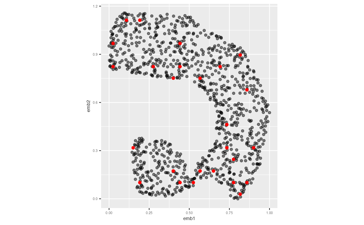
The plot below shows the original UMAP embedding of the training data in grey, overlaid with the predicted 2-D coordinates in red.

umap_scaled <- scurve_model_obj$nldr_obj$scaled_nldr

umap_scaled |>
  ggplot(aes(x = emb1, y = emb2, label = ID)) +
  geom_point(alpha = 0.5) +
  geom_point(data = pred_df_training, aes(x = pred_emb_1, y = pred_emb_2), 
             color = "red", alpha = 0.5) +
  coord_equal() +
  theme(
    plot.title = element_text(hjust = 0.5, size = 18, face = "bold"),
    axis.text = element_text(size = 5),
    axis.title = element_text(size = 7)
  )

Step 3: Computing model summaries

Use the glance() function to compute summary statistics that describe how well the 2-D model captures structure in the high-dimensional space.

glance(
  highd_data = scurve, 
  model_highd = scurve_model_obj$model_highd,
  model_2d = scurve_model_obj$model_2d
)
#> # A tibble: 1 × 2
#>   Error  RMSE
#>   <dbl> <dbl>
#> 1  613. 0.431

Step 4: Augmenting the dataset

To obtain a detailed data frame that includes the high-dimensional observations, their assigned bins, predicted embeddings, and summary metrics, use the augment() function:

augment(
  highd_data = scurve, 
  model_highd = scurve_model_obj$model_highd,
  model_2d = scurve_model_obj$model_2d
) |>
  head(5)
#> # A tibble: 5 × 32
#>      ID      x1    x2       x3       x4       x5      x6       x7 pred_h
#>   <int>   <dbl> <dbl>    <dbl>    <dbl>    <dbl>   <dbl>    <dbl>  <int>
#> 1     1 -0.120  0.819 -1.99     0.0114   0.00351  0.0334  0.00638    200
#> 2     2 -0.0492 0.166  0.00121  0.0115  -0.0166  -0.0297  0.00509    131
#> 3     3 -0.774  0.651  0.367   -0.0172   0.00600  0.0211  0.00303    131
#> 4     4 -0.606  0.952 -1.80     0.0157  -0.00978 -0.0590 -0.00754    227
#> 5     5 -0.478  1.10  -1.88    -0.00423  0.00495 -0.0482 -0.00982    259
#> # ℹ 23 more variables: model_high_d_x1 <dbl>, model_high_d_x2 <dbl>,
#> #   model_high_d_x3 <dbl>, model_high_d_x4 <dbl>, model_high_d_x5 <dbl>,
#> #   model_high_d_x6 <dbl>, model_high_d_x7 <dbl>, error_square_x1 <dbl>,
#> #   error_square_x2 <dbl>, error_square_x3 <dbl>, error_square_x4 <dbl>,
#> #   error_square_x5 <dbl>, error_square_x6 <dbl>, error_square_x7 <dbl>,
#> #   row_wise_total_error <dbl>, abs_error_x1 <dbl>, abs_error_x2 <dbl>,
#> #   abs_error_x3 <dbl>, abs_error_x4 <dbl>, abs_error_x5 <dbl>, …