Getting Started with quollr • quollr

What does quollr do?

Nonlinear dimension reduction (NLDR) methods like UMAP and tSNE can produce very different layouts of the same data depending on method and hyper-parameter choices. Choosing poorly can lead to misleading conclusions, such as spurious clusters or artificial separations between groups. quollr helps you assess which layout most faithfully represents the original high-dimensional structure. It does this by fitting a wireframe model in 2-D and lifting it back into high-dimensional space, where you can inspect it directly using a tour. The result is both a visual diagnostic and a quantitative goodness-of-fit metric (hexbin error, HBE).

Your inputs

The package requires two data objects in a specific format.

library(quollr)

# High-dimensional data: must have an ID column and variables prefixed with x
head(scurve, 3)
#> # A tibble: 3 × 8
#>        x1    x2       x3      x4       x5      x6      x7    ID
#>     <dbl> <dbl>    <dbl>   <dbl>    <dbl>   <dbl>   <dbl> <int>
#> 1 -0.120  0.819 -1.99     0.0114  0.00351  0.0334 0.00638     1
#> 2 -0.0492 0.166  0.00121  0.0115 -0.0166  -0.0297 0.00509     2
#> 3 -0.774  0.651  0.367   -0.0172  0.00600  0.0211 0.00303     3

# 2-D NLDR embedding: must have ID, emb1, and emb2 columns
head(scurve_umap, 3)
#> # A tibble: 3 × 3
#>    emb1   emb2    ID
#>   <dbl>  <dbl> <int>
#> 1 -4.24  5.80      1
#> 2  3.19 -0.851     2
#> 3  4.65 -3.31      3

The ID column links the two datasets. High-dimensional variables must be prefixed with x (e.g. x1, x2, …). The embedding columns must be named emb1 and emb2.

Fit the model in one step

The main entry point is fit_highd_model(), which runs the complete pipeline — scaling, hexagonal binning, centroid triangulation, and lifting into high dimensions — in a single call.

model <- fit_highd_model(
  highd_data = scurve,
  nldr_data  = scurve_umap,
  b1         = 21,
  q          = 0.1,
  hd_thresh  = 0
)

The returned object contains everything needed for visualisation and diagnostics:

model$model_2d — 2-D bin centroids
model$model_highd — high-dimensional bin averages
model$trimesh_data — triangular mesh edges
model$hb_obj — hexagonal bin configurations
model$nldr_scaled_obj — scaled embedding

For a step-by-step explanation of each stage, see vignette("quollr2dataprocessing") through vignette("quollr3hexbin") and vignette("quollr4algo").

Inspect the model in 2-D

The triangular mesh overlaid on the NLDR layout shows how the hexagonal bins are connected. Gaps in the mesh indicate sparse regions in the embedding.

library(ggplot2)

ggplot() +
  geom_trimesh(
    data = model$model_2d,
    aes(x = c_x, y = c_y)
  ) +
  geom_point(
    data = model$nldr_scaled_obj$scaled_nldr,
    aes(x = emb1, y = emb2),
    alpha = 0.4, size = 0.8, colour = "#66B2CC"
  ) +
  theme_linedraw() +
  theme(aspect.ratio = 1)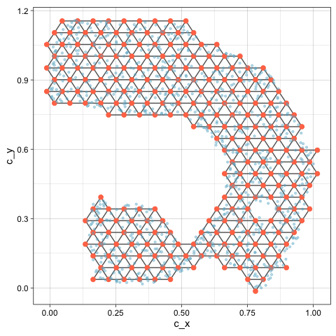

You can also visualise only the hexagonal bins that contain data using geom_hexgrid():

ggplot() +
  geom_hexgrid(
    data = model$model_2d,
    aes(x = c_x, y = c_y)
  ) +
  theme_linedraw() +
  theme(aspect.ratio = 1)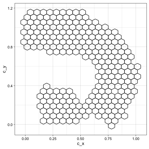

Lift into high dimensions

To inspect how well the 2-D layout preserves the high-dimensional structure, combine the data and model, then view in a tour.

df <- comb_data_model(
  highd_data  = scurve,
  model_highd = model$model_highd,
  model_2d    = model$model_2d
)

# Interactive tour — run this in your R session
show_langevitour(
  point_data = df,
  edge_data  = model$trimesh_data
)

Rotating the tour reveals whether the wireframe traces the true shape of the data in high dimensions. A well-fitted model will follow the data cloud closely across many projection angles. For guidance on interpreting the tour, see vignette("quollr4algo").

Evaluate the fit with HBE

HBE (hexbin error) summarises how well the 2-D layout preserves the high-dimensional structure as a single number — the root mean squared error between the original data and the lifted model.

glance(x = model, highd_data = scurve)
#> # A tibble: 1 × 2
#>   Error   HBE
#>   <dbl> <dbl>
#> 1  196. 0.116

For point-level diagnostics (residuals per observation), use augment():

errors <- augment(x = model, highd_data = scurve)
head(errors[, c("ID", "row_wise_abs_error", "row_wise_total_error")], 5)
#> # A tibble: 5 × 3
#>      ID row_wise_abs_error row_wise_total_error
#>   <int>              <dbl>                <dbl>
#> 1     1             0.210               0.0147 
#> 2     2             0.0955              0.00246
#> 3     3             0.231               0.0128 
#> 4     4             0.206               0.0105 
#> 5     5             0.237               0.0142

Comparing HBE across methods and bin widths helps identify the layout that most faithfully represents the data. See vignette("quollr6bestbinwidth") for guidance on choosing the bin width, and vignette("quollr7bestfit") for a full comparison across NLDR methods.

Linked interactive plots

For deeper diagnostics, quollr provides interactively linked plots that connect the 2-D layout, the high-dimensional tour, and the residual distribution. Brushing in any panel highlights the corresponding points in all other panels.

# Prepare combined data including NLDR coordinates
df_all <- comb_all_data_model(
  highd_data  = scurve,
  nldr_data   = scurve_umap,
  model_highd = model$model_highd,
  model_2d    = model$model_2d
)

show_link_plots(
  point_data  = df_all,
  edge_data   = model$trimesh_data,
  point_colour = "#66B2CC"
)

Where to go next

Vignette	Topic
`vignette("quollr2dataprocessing")`	Data preprocessing and scaling
`vignette("quollr3hexbin")`	Hexagonal binning in detail
`vignette("quollr4algo")`	Full pipeline and tour interpretation
`vignette("quollr5summary")`	Model summaries and residuals
`vignette("quollr6bestbinwidth")`	Choosing the optimal bin width
`vignette("quollr7bestfit")`	Comparing NLDR methods with HBE
`vignette("quollr8linkeddetourr")`	Linked plots with `detourr`